
Proyectos de Investigación en Inteligencia Artificial Aplicada
Section outline
-
AI Research Group
National Technological University
Haedo Regional Faculty
Language
This website is available in English
 and Spanish
  spelling.
Description
The focus of the Artificial Intelligence Research project is on harnessing computer capabilities to enhance human mathematical and logical prowess, as well as automating tasks traditionally performed by humans.
Research objectives
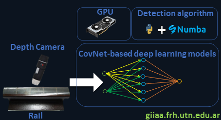
Non-destructive testing of metallic materials using artificial vision can be used in combination with other inspection techniques to decrease diagnostic mistakes. Deep learning, as applied to artificial vision, tries to construct mathematical models that learn from images with cracks or other forms of surface degradation. Because artificial neural networks must process huge amounts of data, very efficient algorithms are required.
Graphical abstract
-
Research and development project
🎙️Gutiérrez
System based on artificial vision cameras for the detection and evaluation of surface defects in metallic materials.
Research objectives
Non-destructive testing using artificial vision on metallic materials can be used in conjunction with other inspection techniques to reduce diagnostic errors. In this sense, deep learning as applied to artificial vision aims to create mathematical models that learn from images that contain cracks or other types of surface damage. The huge amounts of data that artificial neural networks must analyze require the use of highly efficient algorithms. The following objectives were established to respond to these proposals:
General objectives
✅ Create specific algorithms that run on dedicated hardware to detect and evaluate surface defects in metallic materials using the non-destructive testing technique through use of artificial vision.
Specific objectives
✅Establish image processing techniques and deep learning to apply non-destructive artificial vision research.
✅Expand the study of defectology, which the artificial vision method can provide as a necessary complement.
✅Establish the dataset for artificial neural network training.
✅Interpret the results of artificial neuronal network training to predict the defectology under study.
✅Develop programming and implementation skills in the appropriate programming language for the task.

Activities: 0 -
Perceptron
Students involved in the research and development project created a set of examples in Python Jupyter Notebook to show how the perceptron works. They were able to classify logic gates (AND y OR) with two inputs to characterize the perceptron's operation. In this context, they learn artificial intelligence and programming skills while creating content for undergraduate students at the National Technological University - Haedo Regional Faculty..
Activities: 0 -
Introduction
The purpose of this section is to explain the perceptron learning algorithm [1], which was first proposed by Frank Rosenblatt in 1958 and was later refined and thoroughly analyzed by Minsky and Papert [2] in 1969. In addition, the McCulloch-Pitts neural model [3], published in 1943, will be explained, which later evolves into the learning model proposed by [1].
Activities: 0 -
Perceptron evolution
McCulloch-Pitts model
The model proposed by McCulloch-Pitts [3] has a simplified structure and behavior of a physiological neuron, Fig. 1.a, commonly called the bioinspired model. The Biological Neural Network (BRN) has dendrites, which are responsible for receiving stimuli from other neurons, and then transmitting this information to the cell body, regulating its intensity. The cell body is responsible for adding the above characteristics to generate an electrical signal, which, according to the threshold of the action potential given by the different concentrations of Na+, K+ and Cl− ions, generates a trigger towards other neurons. In the case of exceeding the firing potential threshold, the axon transmits the electrical signal generated in the cell body to other neurons through the synapses. The aforementioned mode of operation, by way of example, is artificially replicated by a perceptron, where in figure 1.b the same parts that form part of the biological model can be seen. The Artificial Neural Network (ANN) model consists of inputs (dendrites) that propagate through coefficients (synapses). The linear combination, Eq. 1 (cell body) between inputs and synaptic weights converges in a non-linear operation called activation function (axon).
$$ \color{orange} {S=\sum_{i=1}^{n}{w_i\ast x_i} \quad (1)} $$
A perceptron takes multiple binary inputs, such as x1, x2, and so on, and produces a single binary output. The W coefficients are real numbers that express the contribution of each input to the output. If the sum of the coefficients multiplied by the inputs is greater or less than a certain threshold, the neuron's output will be 1 or 0.
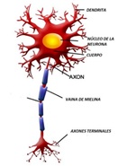
(a) Biological neuron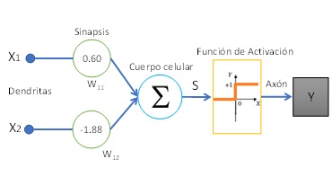
(b) McCulloch-Pitts modelFigure 1: Comparison between a biological and artificial neuron
Activation function proposed by McCulloch-Pitts
Figure 1.b shows that between the exit of the cell body (S) and the exit (Y) there is an activation function (φ(S)). The McCulloch-Pitts mathematical model outputs binary type, labeled {0, 1}. To get the mentioned labels in your output, it is necessary that the activation function has only those possible values. In this sense, the Heaviside function [4], known in this way due to its creator, the mathematician Oliver Heaviside, generates a 0 or a 1 in its output according to the value of S, Eq. 2.
$$ \color{orange} { \varphi\left(S\right) =\begin{cases}1 & S \geq 0\\0 & S <0\end{cases} \quad (2)} $$
Rosenblatt model
Frank Rosenblatt [1] inspired by the work proposed by his colleagues McCulloch-Pitts [3] developed the concept of the perceptron. The perceptron introduces some changes to the model explained in section 2.1. One of the changes he proposes is to introduce an additional input X0 that will have a fixed value of 1 with the coefficient W0. Adding these new parameters is the same as adding a bias to the linear combination of Eq. 1. For this reason, Eq.1 becomes Eq. 3, and as can be seen, the lower limit of the sum starts from i=0.
$$ \color{orange} { S=\sum_{i=0}^{n}{w_i\ast x_i} \quad (3) }$$
The other change made by [1] consists of changing the activation function called the sign function. In this case, the function generates a 0, -1 or 1 in its output according to the value of S, Eq. 4.
$$ \color{orange} {\varphi\left(S\right) =\begin{cases}1 & S>0 \\0 & S=0 \\-1 & S <0\end{cases} \quad (4)} $$Activities: 0 -
Teach To Learn
The perceptron needs to be trained on what to remember to be able to learn. Since the ANN can be trained using a data set to produce the desired output, this type of learning is also known as assisted learning. It is important to note that since this method is for a binary type classification, the input data must be linearly separable. Eq. 5 can be defined to update the synaptic weights W values.
$$ \color{orange} { \mathbf{{W}_{new}} = \mathbf{{W}_{old}}+\mathbf{{Y}_{d}}.\mathbf{X} \quad (5)} $$
\( \color{orange} {\ Donde: \\ \; \\ \mathbf{{W}_{new}} \text{ : Vector of synaptic weights updated} \\ \mathbf{{W}_{old}} \text{ : Vector of prior synaptic weights.}\\ \mathbf{{Y}_{d}} \text{ : Desired output vector.}\\ \mathbf{X} \text{ : Input vector.}} \)
The update rule presented in Eq. 5 is valid if the labels are {-1, 1}. For example, if we have the following scenario:
$$ \color{orange} { \begin{cases}{W}_{0}= 0 +(-1*-1) \\ {W}_{1}=0 +(-1*\;\; 1\;)\end{cases} \quad (6)} $$
Equation (5) is applied for the input and output requirements, and it will allow the coefficients w0 and w1 values to change the direction of the update, Eq. 6. But, in the case that the labels are {0, 1} and there is an incorrect classification of input X and its true value is 0, then the coefficients will never be updated, Eq. 7.
$$ \color{orange} { \begin{cases}{W}_{0}= 0 +(0*1) \\ {W}_{1}=0 +(0*1)\end{cases} \quad (7)} $$
Another updating rule, Eq. 8, can be proposed to solve this inconvenience and to generalize both for -1, 1 and 0, 1 and make it learn.
$$ \color{orange} { \mathbf{{W}_{new}}=\mathbf{{W}_{old}}+(\mathbf{{Y}_{d}-{Y}_{e}}).\mathbf{X} \quad (8)} $$
\( \color{orange} {\ Donde: \\ \; \\ \mathbf{{W}_{new}} \text{ : Vector of synaptic weights updated}\\ \mathbf{{W}_{old}} \text{ : Vector of prior synaptic weights.}\\ \mathbf{{Y}_{d}} \text{ : Desired output vector.}\\ \mathbf{{Y}_{e}} \text{ : Vector of the estimated output}\\ \mathbf{X} \text{ : Input vector.}} \)
The change in Eq. 8 lies in adopting an error that is made up of the difference between the desired output and the corresponding estimated output by combining Eq. 3 and Eq. 2 or Eq. 3 and Eq. 4. In this context, it can be said if the labels are {0, 1}, when the perceptron classifies correctly, the error will be 0. Therefore, it will not be necessary to change the coefficients W. In the scenario where the labels are {-1, 1 }, the error will be 0 if the classification is correct, and in the case of incorrect classification it will be 2 or -2 and the direction of updating the coefficients can be changed.
Activities: 0 -
Loss function
The loss function is employed to determine if the perceptron is learning. If the model's prediction is accurate, this function will have a low value; otherwise, it will have a high value which means that was unable to correctly classify the data. The loss function is zero when the perceptron has learned all of the inputs correctly. The sum of squared errors as expressed in Eq. 9 is a typical loss function.
$$ \color{orange} { \sum_{i=0}^{n}(y_{d_i}-y_{e_i})^2 \quad (9) }$$
\( \color{orange} {\ where: \\ \; \\ y_{d} \ : \ Value \ of \ the \ desired \ output. \\ y_{e} \ : \ Value \ of \ the \ estimated \ output} \)
Activities: 0 -
Python implementation
🎙️Marcelo Gutiérrez
Description
This section provides a brief introduction to the perceptron algorithm and the AND logic gate dataset that we will be using in this tutorial.
Network Initialization
import pandas as pd
import numpy as np

data = [[-1,-1, 1,-1],
        [-1, 1, 1,-1],
        [ 1,-1, 1,-1],
        [ 1, 1, 1, 1]]

pd.DataFrame(data, index=list(range(len(data))), columns=['X1', 'X2','bias','Y'])
Output
### See secction "2.2 Perceptron evolution"###
prediction = sign(np.dot(weight, training))
Activation function
### See secction "2.2 Perceptron evolution"###
def sign(x):
    if x > 0:
        return 1.0
    elif x < 0:
        return -1.0
    else:
        return 1.0
Error of the neural network model
### Ver sección "2.4 Loss function"###
error = desired - prediction
sse += error**2
Weight update
### Ver sección "2.3 Teach To Learn"###
weight = weight + error * training
Algorithm
def sign(x):
    if x > 0:
        return 1.0
    elif x < 0:
        return -1.0
    else:
        return 1.0

import pandas as pd
import numpy as np

data = [[-1,-1, 1,-1],
        [-1, 1, 1,-1],
        [ 1,-1, 1,-1],
        [ 1, 1, 1, 1]]

pd.DataFrame(data, index=list(range(len(data))), columns=['X1', 'X2','bias','Y'])
train_data = pd.DataFrame(data, index=list(range(len(data))), columns=['X1', 'X2','bias','Y'])
train_Y = train_data.Y
train_data = train_data[['X1', 'X2','bias']]
train_data.head()

weight = np.zeros(train_data.shape[1])

for epoch in range(100):
    sse = 0.0
    for sample in range(train_data.shape[0]):
        training = train_data.loc[sample].values
        desired = train_Y.loc[sample]
        prediction = sign(np.dot(weight, training))
        error = desired - prediction
        sse += error**2
        weight = weight + error * training
    print(f'SSE: {sse}')
    if sse == 0:
        break
print(f'Weights: {weight}, Epoch: {epoch+1}')
Activities: 0 -
Referencias
[1] Rosenblatt, F. (1958). The perceptron: A probabilistic model for information storage and organization in the brain. Psychological Review, 65(6), 386–408. https://doi.org/10.1037/h0042519
[2] Minsky, M., Papert, S. (1969). Perceptrons: An Introduction to Computational Geometry, MIT Press, Cambridge, MA, USA. https://doi.org/10.1126/science.165.3895.780
[3] McCulloch, W.S., Pitts, W. A. (1943). Logical calculus of the ideas immanent in nervous activity. Bulletin of Mathematical Biophysics 5, 115–133. https://doi.org/10.1007/BF02478259
[4] Alan V. Oppenheim and Ronald W. Schafer. 2009. Discrete-Time Signal Processing (3rd. ed.). Prentice Hall Press, USA.Activities: 0 -
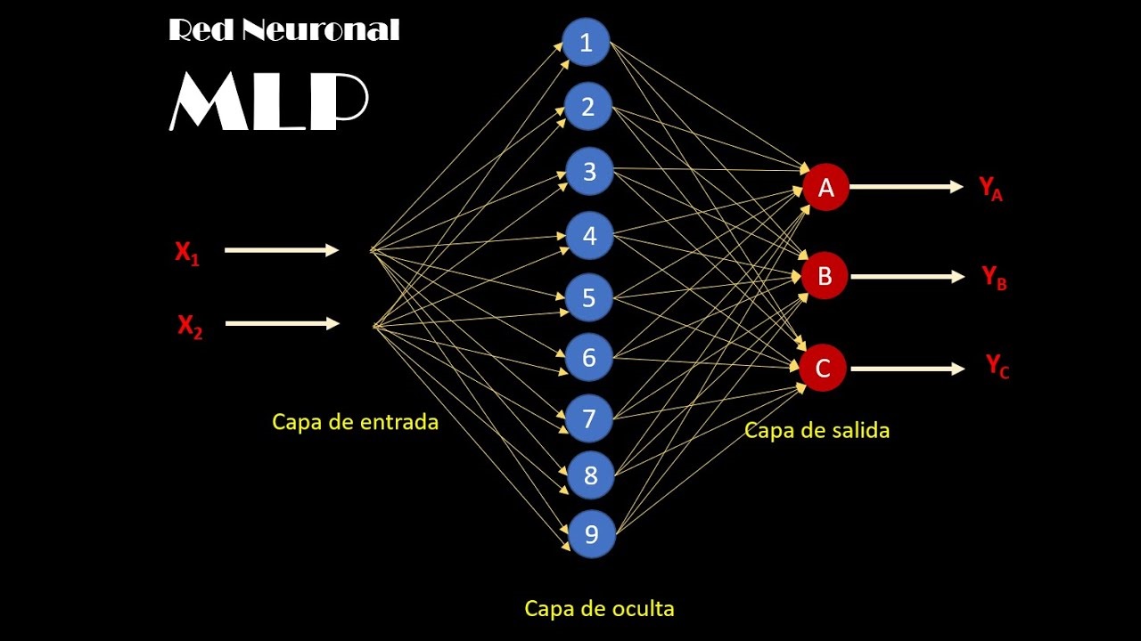
Multilayer Perceptron
 Activities: 0
 -
XOR-Gate with Multilayer Perceptron
🎙️Claudio Acuña
The aim of this example is to learn a two-input XOR logic gate using a fully connected multilayer perceptron. The animation shows how the ANN classifies the inputs labeled as -1,1 based on their output -1,1. Under these conditions, the ANN separates the outputs using decision lines. Backpropagation is the learning algorithm that was used. Students studied the mathematics behind gradient descent to minimize the squared error loss function. In addition, the animation depicts the evolution of the "V" weights in each epoch, which are part of the hidden layer. The objective of the training was to achieve an error of less than 0.05.
Activities: 0 -
MLP regression model
🎙️Marcelo Gutiérrez; Claudio Acuña
Several people think that Artificial Neural Networks (ANN) are "black boxes" but for our team, this is not at all the case. in this video, we explore each stage of an ANN and show the results of training an ANN using a signal as a dataset.
Activities: 0 -
Digital Image Processing
Students involved in the research and development project created a collection of examples in Python Jupyter Notebook to demonstrate digital image processing methods. After reviewing the literature in this field, the students implement color space transformations and filtering using convolution kernels. In this context, they learn digital image processing and programming skills while creating content to share with undergraduate students National Technological University - Haedo Regional Faculty..
Activities: 0 -
YIQ color space
🎙️Claudio Acuña
Digital image processing frequently makes use of the YIQ color space. One of the reasons is the possibility for recovering the Y component, which is associated with the grayscale image.
Activities: 0 -
Image Kernels
🎙️Marcelo Gutiérrez; Claudio Acuña
An image kernel is a tiny matrix that is used to create effects similar to those seen in Photoshop or Gimp, such as blurring, sharpening, outlining, and embossing. They are also used in machine learning for 'feature extraction,' which is a method for detecting the most relevant parts of a picture. In this context, the process is known more broadly as convolutional neural networks (ConvNet).
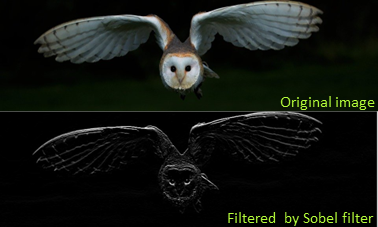
Sobel filter
Edges are abrupt discontinuities in an image that can be caused by surface color, depth, illumination, or other factors. In this sense, we identify the edges in the image below wherever there is a sudden change in intensity.
 Activities: 0
 -
Convolutional neural networks
En este video, creado por los integrantes del proyecto de investigación y desarrollo, explora el funcionamiento de una red neuronal convolucional desarrollada desde cero para el conjunto de datos MNIST. Tras programar cada etapa, los estudiantes comparten cómo funciona el entrenamiento para dígitos escritos a mano.
Stride
"Stride" en una red neuronal se refiere a la cantidad de pasos que toma el filtro o la ventana de convolución al moverse a través de la entrada. Un "Stride" más grande significa que el filtro se desplaza en incrementos mayores, reduciendo la resolución espacial de la salida y acelerando el proceso de convolución.
Cross-Correlation
Cross-Correlation" es un paso esencial en la convolución de redes neuronales. Representa la comparación punto a punto de dos conjuntos de datos, como un filtro y una porción de entrada. Este proceso destaca la presencia de patrones específicos y ayuda a la red a reconocer características importantes en los datos.
Max Pooling
"Max Pooling" es una técnica utilizada para reducir la dimensionalidad de una capa de convolución, conservando las características más relevantes. Consiste en seleccionar el valor máximo de una región específica de la capa de entrada. Esto ayuda a disminuir la carga computacional y a mejorar la invarianza a pequeñas traslaciones en la entrada.
Activities: 0 -
Algorithms
This research project use Google Colab to run the algorithms.
Model Description Google Colab Perceptron The perceptron is a simplified model of a biological neuron 🚫 MLP A multilayer perceptron is a feedforward artificial neural network model that maps sets of input data onto a set of appropriate output MLP with Backpropagation 🚫 Activities: 0 -
Graduate students
Claudio Acuña Pavese, 2022, “Thickness gauge using the eddy current method”.
Technical summary
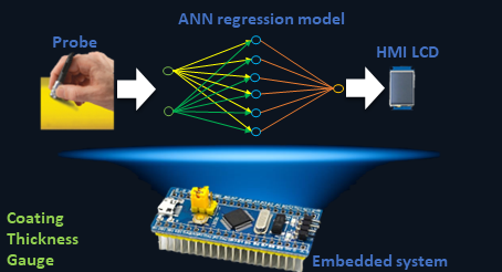
Non-destructive testing (NDT) by eddy currents (EC) is a reliable evaluation method that is applied in different areas such as nuclear, the petrochemical industry, air and rail transport, among others. The wide use of coating meters is known, both in different industries and in research and development laboratories. Generally, these devices are manufactured to perform measurements on a limited number of substrates, reducing the range of applications. In this context, the project aims to develop and implement artificial neural network (ANN) algorithms and build a functional prototype for field application in an embedded system. The sensor is composed of a Colpitts oscillator. The impedance of the resonator tank is modified according to the lift-off (in EC lift-off is called the separation between the probe and the component to be inspected), and this generates changes in the resonance frequency. The system calibration curve is determined through the variation of the resonance frequency as a function of the lift-off. Eddy currents method, like all NDT methods, is a comparative method that needs a calibration curve in order to be implemented. The sinusoidal signal coming from the probe enters the embedded system that will be in charge of conditioning it. In the next stage of the device, a calibration must be performed depending on the substrate being used. Calibration is performed by training an ANN, which will have the output frequency of the oscillator as data set according to the thickness of standard gauges. In the last stage, the trained ANN will return the value of the coating thickness and this parameter will be displayed on an HMI interface or screen. The system will be powered by a rechargeable battery and recharging will be through an external power supply. The portable device must work with thicknesses between 25 and 905 microns on 6061 aluminum and Zry-4. Consequently, this project will contribute to the research and development group "Non-destructive testing applied to the railway industry" of the Haedo Regional Faculty and to the industry that uses this measurement technique.
Graphical abstract
Activities: 0 -
Location
AI Research Group
National Technological University
Haedo Regional Faculty
532 Paris Street
Buenos Aires, Argentina
Phone: +54-011-4443-7466 (ext. 144)
Fax: +54-011-4443-0499
Website: giiaa.frh.utn.edu.arActivities: 0