
2.2 Perceptron evolution
Perfilado de sección
-
Evolución del perceptrón
Modelo McCulloch-Pitts
El modelo que propone McCulloch-Pitts [3] tiene una estructura y comportamiento simplificado de una neurona fisiológica, Fig. 1.a, comúnmente llamado modelo bioinspirado. La Red Neuronal Biológica (RNB) presenta dendritas, que son las encargadas de recibir los estímulos de otras neuronas, luego trasmite esta información al cuerpo celular regulando su intensidad. El cuerpo celular se encarga de sumar las características anteriores para generar una señal eléctrica, que de acuerdo con el umbral del potencial de acción dado por las diferentes concentraciones de iones Na+, K+ y Cl− genera un disparo hacia otras neuronas. En el caso de superar el umbral del potencial de disparo, el axón transmite la señal eléctrica generada en el cuerpo celular a otras neuronas a través de las sinapsis. El modo de funcionamiento antes mencionado, a modo de ejemplo, es replicado por un perceptrón en forma artificial, donde en la figura 1.b se puede ver las mismas partes que forman parte del modelo biológico. El modelo de Red Neuronal Artificial (RNA) consiste en entradas (dendritas) que se propagan por los coeficientes (sinapsis). La combinación lineal, Ec. 1 (cuerpo celular) entre las entradas y los pesos sinápticos confluye en una operación no lineal denominada función de activación (axón).
$$ \color{orange} {S=\sum_{i=1}^{n}{w_i\ast x_i} \quad (1)} $$
Un perceptrón toma varias entradas binarias x1, x2, etc y produce una sola salida binaria. Los coeficientes W son números reales que expresa la importancia de la respectiva entrada con la salida. La salida de la neurona será 1 ó 0 si la suma de la multiplicación de los coeficientes por entradas es mayor o menor a un determinado umbral.
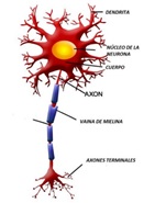
(a) Neurona biológica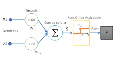
(b) Modelo McCulloch-PittsFigura 1: Comparación entre una neurona biológica y artificial
Función de activación propuesta por McCulloch-Pitts
En la figura 1.b se aprecia que entre la salida del cuerpo celular (S) y la salida (Y) existe una función de activación \( (\varphi\left(S\right)) \) $$ \color{orange} { \varphi\left(S\right) =\begin{cases}1 & S \geq 0\\0 & S <0\end{cases} \quad (2)} $$
Modelo Rosenblatt
Frank Rosenblatt [1] inspirado en el trabajo propuesto por sus colegas McCulloch-Pitts [3] desarrollo el concepto de perceptrón. El perceptrón introduce algunos cambios al modelo explicado en la sección 2.1. Uno de los cambios que propone es introducir una entrada adicional X0 que tendrá un valor fijo en 1 con el coeficiente W0. Al adicionar estos nuevos parámetros es lo mismo a agregar un sesgo a la combinación lineal de la Ec. 1. Por tal motivo, la Ec.1 se convierte en la Ec. 3, y como se observa el limite inferior de la sumatoria comienza desde i=0.
$$ \color{orange} { S=\sum_{i=0}^{n}{w_i\ast x_i} \quad (3) }$$
El otro cambio que realiza [1], consiste en cambiar la función de activación denominada función signo. En este caso, la función genera un 0, -1 o 1 en su salida de acuerdo con el valor de S, Ec. 4.
$$ \color{orange} {\varphi\left(S\right) =\begin{cases}1 & S>0 \\0 & S=0 \\-1 & S <0\end{cases} \quad (4)} $$